Agile Visualization

Visualizing Polymetric Graphs using Mondrian

Mondrian is a rich API which offers facilities to describe and render graphs. Mondrian is an essential piece of Roassal due to its expressiveness and simplicity of use. For any data structure, Mondrian allows mapping of metric values and properties into visual dimensions, such as shape and colors.

Mondrian is often considered as being the most expressive part of Roassal: highly interactive and flexible visualizations may be the result of just a few lines of code. Mondrian is often the starting point of the Roassal platform.

An online video illustrates this chapter: http://bit.ly/Mondrian-AgileVisualization

1. A first visualization

As a contrived example, consider the following script (Figure 1.1):

	b := RTMondrian new.
	b nodes: #('hello' 'world' 'bonjour' 'tout le monde' 'Guten' 'Morgen').
	b

Six gray squares are horizontally lined up. Each square corresponds to a word contained in the array passed to nodes:. Several layouts are available, thanks to the layout builder (see the description of the layout builder in the Layout chapter). For example, the force layout is activated as:

	b := RTMondrian new.
	b nodes: #('hello' 'world' 'bonjour' 'tout le monde' 'Guten' 'Morgen').
	b layout force.
	b

Edges may be simply added using the edge builder, accessible by sending edges to the Mondrian builder:

	b := RTMondrian new.
	b nodes: #('hello' 'world' 'bonjour' 'tout le monde' 'Guten' 'Morgen').
	b shape line.
	b edges useAssociations: { 
		'hello' -> 'world' .
		'bonjour' -> 'tout le monde' .
		'Guten' -> 'Morgen' }.
	b layout force.
	b

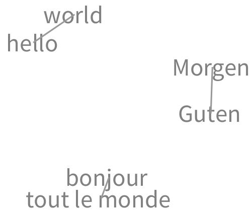
A label may be used instead of a grayed box and the layout may be configured as follows (Figure 1.2):

	b := RTMondrian new.
	b shape label.
	b nodes: #('hello' 'world' 'bonjour' 'tout le monde' 'Guten' 'Morgen').
	b shape line.
	b edges useAssociations: { 
		'hello' -> 'world' .
		'bonjour' -> 'tout le monde' .
		'Guten' -> 'Morgen' }.
	b layout force charge: -200.
	b

As a slightly more elaborated example, consider the following example:

	b := RTMondrian new.

	b nodes: (1 to: 300).
	b edges connectFrom: [ :value | value // 2 ].

	b shape 
		bezierLineFollowing: [ :value | value // 2 ];
		color: Color blue trans.
	b edges 
		notUseInLayout;
		connectTo: [ :value | (value / 10) asInteger + (value \\ 10) ].

	b layout cluster.
	b

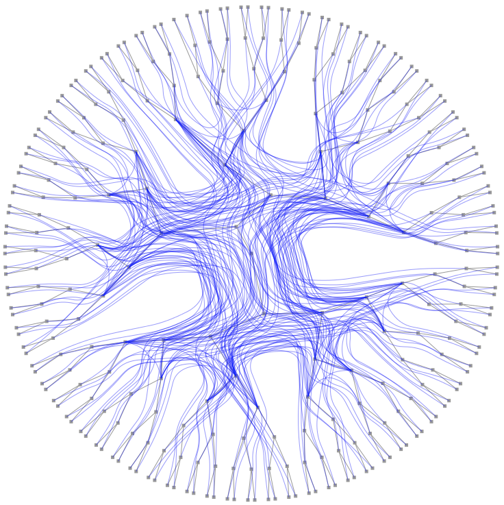
1.3. Visualizing numbers and their connections

The example creates an instance of the class RTMondrian and assigns this object to the b variable. Nodes are then set in the builder, which are 300 successive numbers, starting from 1. Each node is represented as a little gray square. Two sets of edges are defined. The first set, described using b edges connectFrom: [ :value | value // 2 ], models the relation between a value and value // 2. The message // returns "the integer quotient defined by division with truncation toward negative" as indicated by the comment of the method // defined in the class Number (e.g., 9//4 = 2).

The second set of edges, described using b edges notUseInLayout; connectTo: [ ... ], is defined as the sum of the two digits. For a given numerical value, the expression (value / 10) asInteger returns the first digit or it and value \ 10 the last digit. Each number is linked to another number representing the sum of its digits (e.g., 15 is linked to 6). These edges are not taken into account for the layout as specified with the message notUseInLayout.

The first set of edges uses the default shape for lines, which is straight, gray, and non-directed. For the second set, a shape is defined as a Bezier line following the control points given by the expression value // 2, painted in a translucent blue.

The layout used is cluster, forming a radial-like appearance. For this set of elements and edges, horizontalTree, tree, radial are all relevant layouts.

2. Visualizing CSV data

The previous examples visualized numerical values and define some connections based on a mathematical relation. Any arbitrary objects may be visualized with Mondrian. Consider the following example that displays data obtained from a CSV (comma separated file):

"You need to load the plugin Neo JSON and CSV parser, available from the World menu"
csvContent := 
'Santiago,5.1,Chile
Valparaiso,0.5,Chile
Paris,2.2,France
Nice,0.7,France,
Chile,16,
France,66,'.
values := (NeoCSVReader on: csvContent readStream) upToEnd.

b := RTMondrian new.
b shape circle 
  size: [ :aName |  
   (Float readFrom: (values detect: [ :a | a first = aName ]) second) log * 30 ];
  withTextAbove.

b nodes: (values collect: #first).
b edges connectFrom: [ :aName | (values detect: [ :a | a first = aName ]) third ] .
b layout tree.
b

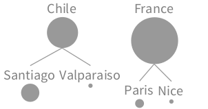
Figure 2.1 illustrates the result. Data obtained from a CSV description is used in the visualization. Each city and country is represented as a circle. The size of the circle represents the number of people living in the city or the country. We use a logarithmic scale to cope with large variations.

To keep the example concise and self-contained, the CSV content is provided as a Pharo String. If you wish to have the file externally provided, then you may simply have

	csvContent := 'file.csv' asFileReference contents.
	values := (NeoCSVReader on: csvContent readStream) upToEnd.
	...

In that case, a file named file.csv has to be in the same folder as your Pharo image. A full path may be provided.

3. Mondrian Script Structure

As illustrated in the example given above, a script in Mondrian essentially contains five different sections: shape description, node declaration, edge declarations, layout description, normalization.

The message shape, layout, edges sent to an RTMondrian object returns a shape, layout builder, and edge builders, respectively. Sending the message nodes: creates some elements using the shape previously defined.

4. Visualizing Software

As a first example, consider the following script (Figure 4.1):

	b := RTMondrian new.
	b shape rectangle
		withBorder;
		width: [ :cls | cls numberOfVariables * 5 ];
		height: [ :cls | cls numberOfMethods ].

	b nodes: Collection withAllSubclasses.
	b edges connectToAll: [ :cls | cls subclasses ].
	b layout tree.
	b normalizer
		normalizeColorAsGray: [ :cls | cls numberOfLinesOfCode ].
	b

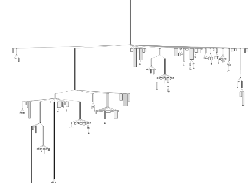
The script visualizes the collection class hierarchy obtained with the expression Collection withAllSubclasses. Relation between nodes is obtained by linking each nodes to its subclasses. A tree layout is then set.

Each box of the visualization represents a class. The height of a class indicates its amount of methods that it defines. The width indicates the number of variables the class defines. The color indicates the number of lines of code the class defines (white = the class with the smallest number of lines of code, black = the heaviest class). Each of Mondrian node is draggable and has a tooltip.

The normalizer may also give a particular color to an element based on an attribute or a property. Consider the following example (Figure 4.2):

	b := RTMondrian new.
	b shape circle.
	b nodes: Collection withAllSubclasses.
	b shape line color: Color veryLightGray.
	b edges 
		moveBehind;
		connectFrom: #superclass.
	b layout cluster.
	b normalizer
		normalizeSize: #numberOfMethods min: 6 max: 40;
		distinctColorUsing: #package.
	b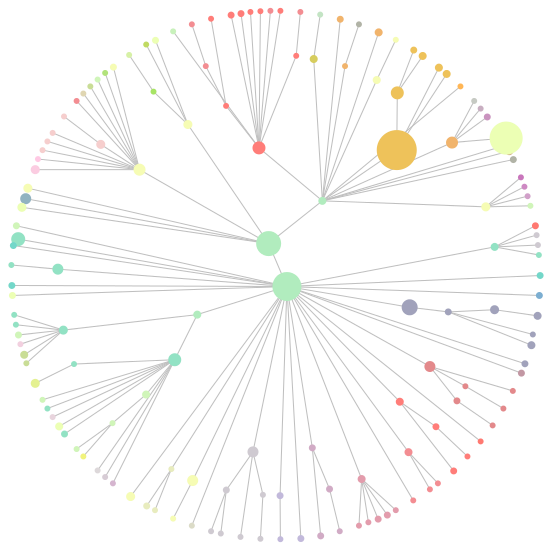

4.2. Each circle is a class and its color indicates the class packages

The script simply associates a circle to each class, subclass of the class Collection. Edges indicates superclass links. The cluster layout makes subclasses located around a superclass. Each class has a color, representing the package of a class. Each package has a color, given by the message distinctColorUsing:.

5. Nesting

Mondrian offers a convenient way to nest elements. Each node may act as a space to which nodes may be added. The message nodes:forEach: has to be used for that purpose. Consider the following example (Figure 5.1):

	b := RTMondrian new.
	b nodes: (0 to: 90 by: 10) forEach: [ :each | 
		b nodes: (1 to: each).
		b layout grid
	].
	b layout flow.
	b

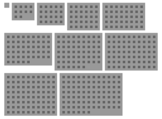
There are 10 top level nodes, representing the values 0, 10, 20, ..., up to 90. Each node contains an amount of inner values that correspond to the number it represents.

Encapsulating nodes may also have a title and be connected (Figure 5.2):

	b := RTMondrian new.
	b shape rectangle withTextAbove.
	b nodes: RTShape withAllSubclasses forEach: [ :class |
		b nodes: class methods.
		b layout grid.
	].
	b edges connectToAll: #subclasses.
	b layout tree.
	b

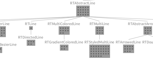
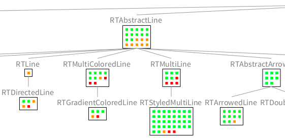
The use of withTextAbove makes each encapsulating node have a title above. Node color may be set to reflect particular conditions, as in the following example (Figure 5.3):

	b := RTMondrian new.
	b shape rectangle withTextAbove; 
		fillColor: Color white; borderColor: Color black.
	b nodes: RTShape withAllSubclasses forEach: [ :class |
		b shape rectangle
			if: [ :m | m numberOfLinesOfCode < 5 ] fillColor: Color green;
			if: [ :m | m numberOfLinesOfCode >= 5 ] fillColor: Color orange;
			if: [ :m | m numberOfLinesOfCode >= 10 ] fillColor: Color red.
		b nodes: (class methods sortedAs: #numberOfLinesOfCode).
		b layout grid.
	].
	b edges connectToAll: #subclasses.
	b layout tree.
	b

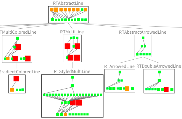
Inner nodes may have a proper shape and be connected. Consider the following version of the visualization of the Roassal shapes (Figure 5.4):

	b := RTMondrian new.
	b shape rectangle withTextAbove; 
		fillColor: Color white; borderColor: Color black.
	b nodes: RTShape withAllSubclasses forEach: [ :class |
		b shape rectangle
			if: [ :m | m numberOfLinesOfCode < 5 ] fillColor: Color green;
			if: [ :m | m numberOfLinesOfCode >= 5 ] fillColor: Color orange;
			if: [ :m | m numberOfLinesOfCode >= 10 ] fillColor: Color red;
			size: [ :m | m numberOfLinesOfCode sqrt * 5 ].
		b nodes: class methods.
		b edges connectToAll: #dependentMethods.
		b layout sugiyama.
	].
	b edges connectToAll: #subclasses.
	b layout tree.
	b

6. Visualizing File and Directories

File systems have a hierarchy driven by the nesting of folders and files. Consider the following code:

	fr := UIManager default chooseDirectory.
	fr ifNil: [ ^ self ].
	allChildren := fr allChildren.
	allChildren := allChildren copyWithout: fr.

	b := RTMondrian new.

	b nodes: fr children forEach: [ :fileRef |
		b shape box 
			size: [ :f | (f size + 1) log * 3 ].
		b nodes: fileRef allChildren.
		b edges connectFrom: #parent.
		b layout tree.

	].
	b layout verticalLine.
	b normalizer
		objects: allChildren;
		distinctColorUsing: #extension.

	b

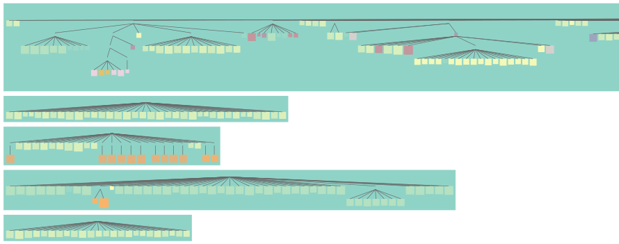
The instruction UIManager default chooseDirectory opens a file browser to let the user (i.e., you) select a directory. The class UIManager offers many methods to require input from the user. The message allChildren, sent to the FileReference returned by chooseDirectory, returns a collection of all the file references. For each file directly contained in the selected directory, a hierarchy is shown. The size of a box representing a file depends on the number of characters contained in that file. A logarithmic scale is used to cope with file size disparities. Thanks to the GT infrastructure, clicking on a file displays its content.